S3.4 Generalized governing equations in LMP

Laser machining processes have found wider and wider applications in the past few decades. Laser machining is assumed to be flexible, rapid and precise. However, process parameters such as laser intensity, laser beam size, laser pulse duration, depth of focus, beam quality, and scanning speed of the laser source must be carefully selected for each application to achieve optimized results. While empirical knowledge and experience have historically been employed to determine the process parameters, there has been continuous efforts in quantitatively relating the physics of laser machining process with the process parameters. The modeling of the laser machining process is a critical element for its successful operation, and these models can contribute a lot to the control and optimization of the process.

It is realized that laser machining processes are complicated due to their wide range of laser intensity, laser-material interaction time, scanning speed, beam size and wavelength. At an energy intensity of the order of 10³ to 10⁴ W/cm², heat conduction and solute diffusion are dominant in determining the dwell time required for phase transformation in laser surface hardening. When laser intensity goes up to 10⁷ W/cm² level, as in laser deep penetration welding, conduction, convection, evaporation and plasma interaction all com to play an important role in the process. In laser machining, the energy level covers 10⁶ to 10⁹ W/cm². In this energy range, conduction, convection, evaporation, plasma generation, gas dynamics and gas jet effects are important. With the development of ultrashort ( <10 psec) pulse lasers, the energy levels are further expand to 10¹², the interaction mechanism is quite different because of the short pulse duration time.

As mentioned before, many models has been suggested, both analytical and numerical. Early models were mostly analytical in nature and primarily describe the conductive thermal fields induced in the solid by a moving laser source. The temperature dependent nature of the physical properties involved in the models and the complex geometry in reality make it necessary for numerical solutions.

The laser machining process is complex, so many models have been suggested, can we extract some general information from the existing works?

It is the purpose of this section that a general model be presented to give the reader an overall understanding of the laser machining processes.

In Section 3.4 Level 2 we have reviewed the basics of heat transfer and fluid mechanics. In laser machining process, the convection as well as the diffusion of the energy field should be considered. Thus the heat conduction equation should be replaced by the more general energy equation. Then the heat transfer analysis and the fluid motion analysis of the process become coupled together. The governing equations describing the laser machining process in the target material (We are not considering the gas dynamics and plasma interaction) are the Continuity equation, Momentum equation, and Energy equation.

We list them here for convenience, for details please refer to Section 3.4 Level 2.

General equation of heat conduction:

Continuity equation:

Momentum equation:

Energy equation:

The properties involved may be temperature or pressure dependent, they may be highly non-linear. To build a model for numerical solutions, we are facing the task of writing programs to implement the governing equations for specific calculation domains. It is highly desirable if a general algorithm can be applied to the above equations. There are common features in the above equations which make a generalization possible. In a word, all the equations can be generalized as Transport Equations.

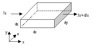
Figure 3.58 illustration of net flux into a control volume

Every differential equation represents a kind of conservation. Every term in the equation represent a volume based effect. Let J be the flux of variable , we consider the control volume dx, dy, dz in figure 3.58. Jx is the flux into left face with an area dydz, the right face leaving flux is . So the net flux is . The net flux in y and z direction can be considered in the same way. Then we have the net flux for the control volume is:

The net flux can be divided into convection and diffusion part and be expressed as:

where u is velocity field and is the diffusion coefficient.

The unit volume rate of change of variable is.

Then the general transport equation is:

where S is the source term. The four terms in the above equation represent the transient term, convection term, diffusion term and source term. The differential equation simply expresses the conservation of the dependent variable in the control volume. can be various physical properties, such as enthalpy, temperature, mass, velocity, etc. One can easily verify that the equations we mentioned in fluid mechanics and heat transfer can all be transformed in the general transport equation. During the transformation, one has to decide the correspondent coefficients and the source term. All terms besides the rate term, convection and the diffusion term are ascribed to the source term.

For example, the momentum equation in x-direction is:

The above conservation equation is derived from coordinates fixed on the substrate (x₀, y₀, z₀). When the scanning of the laser source is considered, a coordinate transformation is needed for convenience. Suppose laser source has a scanning speed in x-direction U_s relative to the substrate, and define the coordinate system fixed to the laser beam to (x, y, z), we have:

and for constant scanning velocity.

Also:

Taking these relations into the general equation, the equation fixed on laser source can be derived.

Having got the general form of the governing equation, the next task is how to discrete the equation and write the program. We won't go to further detail for this part, since there are good references on this topic, and there are too much contents to cover to make it clear. We see the possibility of writing a general program and use them for different processes.

The final form of the discretized equations all takes the following form:

This equation says the point p value is related to its neighboring values and the residual term b. The coefficients and b are decided according to certain discretization criteria.

Combining the boundary conditions and initial conditions, the group of equations can be solved. In the programming, the non-linearity of the property are considered using certain linearization approximations or using iterations. The book of Patankar is highly recommended for readers who want to write programs to solve own problems.

References:

Suhas V. Patankar, 1980, Numerical Heat Transfer and Fluid Flow, McGraw, new York, 1980.

J. Mazumder, P.S. Mohanty and A. Kar, "Mathematical modelling of laser materials processing," 1996, Int. J. of Materials and Product Technology, Vol. 11, pp.193-252.

Frank, P. I. and David P. D., 1996, Fundamentals of Heat and Mass Transfer, John Wiley & Sons, Inc., 4th edition, New York.

Frank, M. W., 1999, Fluid Mechanics, WCB/McGraw-Hill, 4th edition, New York.