![]()
![]()
S3.2 Boundary conditions in modeling
Specifying the suitable boundary conditions is the basis for successful computation. In this section we first discuss some general aspects of boundary conditions, then we use them for the laser machining processes.
Heat transfer boundary conditions:
Three kinds of boundary conditions are typically encountered in heat conduction analysis, these are:
Given the boundary temperature T,
Given the boundary heat flux q, and
Given a boundary heat flux balance relation.
If the boundary temperature is given, there is no particular difficulty in modeling, one needs only specify the value of the boundary grids to the specified temperature.
If the boundary heat flux along direction x is given, the energy balance is:
![]()
where q is the boundary heat flux, k is the heat conductivity, T is temperature.
The more general case is a boundary energy balance relation. For example, sometimes the boundary inward heat flux q is specified in terms of a heat transfer coefficient h and a surrounding temperature Tf . Then the boundary condition is:
![]()
The above relation is the energy balance between boundary heat conduction and the boundary heat convection. If radiation and heat flux should also be considered, we have the following boundary conditions:
![]()
where ![]() is Stefan-Boltzmann
constant,
is Stefan-Boltzmann
constant, ![]() is the surface
emissivity. This relation can be used to model simple 1D heat transfer in laser
heat treatment if one specify qin to be the absorbed laser
energy.
is the surface
emissivity. This relation can be used to model simple 1D heat transfer in laser
heat treatment if one specify qin to be the absorbed laser
energy.
Note that the above boundary conditions consider no effect of phase change. But in laser machining, phase change effect can not be neglected. To consider the phase change effect, the boundary mass flow qmass (define leaving flux to be positive) must be known, then one can include the energy brought away by the mass flux. Let the energy brought away by unit mass to be e, the boundary condition is:
![]()
The energy brought away by unit mass is consisted of internal energy eint and kinetic energy ek. The mass flow is related to the surface recessing velocity vn during machining. So we have:
![]()
It is clear that to deal with phase change problems, the properties at the solid-liquid-vapor interface must be studied in detail. The properties involved include interface temperature, particle velocity relative to the target, surface recessing velocity, latent heat, etc. This topic will be discussed in following sections, Section 3.5 and Section 3.6.
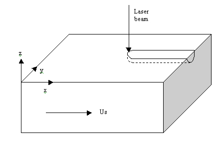
Figure 3.51: The configuration of laser machining process
 Example: In laser
machining, as illustrated by Fig. 3.51, the laser beam is applied on the top
surface of the target, a groove is formed when the laser scans across the target.
Derive the boundary conditions for heat transfer modeling, neglecting radiation
and convection effects.
Example: In laser
machining, as illustrated by Fig. 3.51, the laser beam is applied on the top
surface of the target, a groove is formed when the laser scans across the target.
Derive the boundary conditions for heat transfer modeling, neglecting radiation
and convection effects.
Solve:
Assuming the convection effect of the liquid material can be neglected, the governing equation is the heat conduction equation:
![]()
The temperature far away from the scanning point is at room temperature, and on the top groove surface z = S(x,y), an energy balance relation should be considered. Let n be the groove normal direction, vn be the surface recessing velocity along the normal direction. The boundary conditions are:
![]()
and at z = S(x,y),
![]()
Fluid flow boundary conditions:
In Level 2 Section 3.4 we have reviewed the basic fluid mechanics. The fluid flow boundary conditions are described here. The boundary conditions we are considering are solid-liquid interface, inlet and outlet , and the liquid-gas interface or the free surface.
Fig. 3.52 shows an SEM picture of a laser drilled hole on pure copper using 50 pulses at 6e8 W/cm2 laser intensity, laser pulse duration time is 50ns, beam size is 4.5microns. The flow of molten layer is obvious. So the fluid flow boundary condition is also needed for laser machining processes.
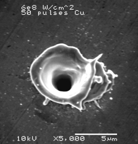
Figure 3.52: UV Laser machining of copper at ns time scale show clear indication of fluid motions.
First, for a solid, impermeable wall, there is no slip and no temperature jump between a viscous heat conducting fluid and the solid
Vfluid=Vwall and Tfluid=Twall for solid wall
This boundary condition applies for laser machining when the dynamic motion of the molten layer is considered.
The second kind of boundary is the inlet or outlet boundary condition. The complete distribution of pressure, velocity, and temperature must be known at all times at inlet or outlet:
Kown V, P, T at inlet or outlet
However the outlet distributions of the variables are usually unknown in practice, sometimes they should be the results of calculation, while the inlet flow is usually given. Then what shall we do with the outlet boundary condition when calculating the fluid field numerically? The answer is surprisingly simple: No boundary condition information is needed at the outflow boundary as long as the Peclet number is sufficiently large.
Peclet number is defined as:
![]()
where V is the flow velocity, L is the characteristic length
of the flow field, ![]() is
the diffusion coefficient. Peclet number is the ratio of the strengths of convection
and diffusion. So if Peclet number is large enough, the influence of downstream
to the calculation domain can be neglected.
is
the diffusion coefficient. Peclet number is the ratio of the strengths of convection
and diffusion. So if Peclet number is large enough, the influence of downstream
to the calculation domain can be neglected.
The third and the most complex conditions occur at a liquid-gas interface. The liquid and the gas velocity at this interface must be equal, this is called the kinetic boundary condition:
Vliq=Vgas
There must be mechanical equilibrium across the interface as well. The viscous-shear stress must balance:
![]()
Also the pressure must balance the surface tension effect at the interface:
![]()
where ![]() is the surface tension
coefficient, Rx and Ry are the liquid surface curvature radius
along the x, y direction respectively.
is the surface tension
coefficient, Rx and Ry are the liquid surface curvature radius
along the x, y direction respectively.
And finally the energy balance at the liquid-gas interface should be considered, which has been discussed in the heat transfer part.
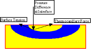
Figure 3.53 Boundary conditions in fluid flow analysis of laser machining process
In laser machining, a thin layer of liquid material may exist such as laser metal machining. In this case, thermocapillary convection or Marangoni Mechanism becomes important. When the surface tension variations arise due to temperature gradients along the interface, the shear stress acting on the interface induce fluid motions. This effect is especially important for laser welding processes when the dynamics of the welding pool has to be analyzed. This effect is also used to explain the surface morphology of the laser-induced bumps and fluid motion in laser drilling.
In this case the force balance boundary condition along the surface normal direction is:
![]()
where ![]() is the surface
normal,
is the surface
normal, ![]() is the surface
tangential unit vector. This equation states: at the free surface, vaporization
recoil pressure, surface tension and thermocapillary force are balanced.
is the surface
tangential unit vector. This equation states: at the free surface, vaporization
recoil pressure, surface tension and thermocapillary force are balanced.
We won't go into details for this part due to limited time and contents requirements. Interested reader can refer to relevant literatures.
References:
Balandin, Y. V., et al., 1995, "Thermocapillary flow excited by focused nanosecond laser pulses in contaminated thin liquid iron films." Journal of Appl. Phys., Vol. 78, pp.2037-2951.
Bennett, T.D., et al., 1997, "Marangoni Mechanism in Pulsed Laser Texturing of Magnetic disk substrates," J. Heat Transfer, Vol. 119, pp. 589-596.
Frank, P. I. and David P. D., 1996, Fundamentals of Heat and Mass Transfer, John Wiley & Sons, Inc., 4th edition, New York.
Frank, M. W., 1999, Fluid Mechanics, WCB/McGraw-Hill, 4th edition, New York.