S3.4 Introduction of LMP modeling

We have discussed how to describe laser energy and how laser energy is absorbed by target material. Now we move onto the discussion of modeling of Laser Machining Process. You may ask, what is the purpose of modeling?

Well, it is may be fun to just look at the process, but as engineer we must know the accuracy of the process and we need to control the machining tolerances. So the purpose of modeling and simulation is as following:

1. Quantitatively understand the process, use these information as guidelines for machining process estimation and control;
2. Parametric optimization of laser machining process. There are many operation parameters in laser machining process, for example, laser power, focus spot size, wavelength, stand off distance, jet pressure, etc., to make the process more accurate and more consistent, modeling and simulation is the powerful tool besides experimental exploration;
3. Using modeling and simulation to reveal the physical processes in depth and in detail. Some aspects of the physical process are difficult or impossible to study through pure experimental techniques. For example, the temperature distribution and temporal evolvement in target material, the coupling of laser energy with cavity profile, the residual stress distribution, etc.

CAD/CAM/CAE has made great contribution to modern science and engineering, Modeling and simulations are such efforts in the realm of laser machining process.

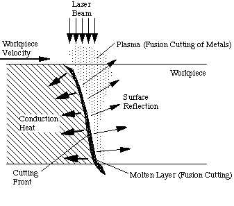
Figure 3.7 Phenomena in laser cutting

Next let's look at the physics involved in modeling of laser machining process. Laser machining is mainly a thermal-mechanical process, material is removed through phase changes (melting and/or vaporization) and hydrodynamic motions (gas jet blowing and hydrodynamic ablation). Many other processes are involved, such as plasma generation, shock wave generation, etc.

Thus heat transfer, fluid mechanics and gas dynamics as well as plasma physics are all topics of modeling. Wow! This is scaring! It is true that laser material interaction is a complex process, many researchers are still working on it, on the other hand, this indicates that the theoretical aspect of laser machining is not fully developed. Laser machining process is said to have many advantages over traditional machining processes, but it needs the accumulation of numbers and laws to make it more accurate, more controllable and more promising.

These models can be divided into two kinds, one is model having analytical solutions, the other is model having numerical solutions only. A lot of stuff should be studied in this area. We will move on step by step, in Level one, you need only to understand the one dimensional stationary heat conduction model. For advanced knowledge of modeling, please go to chapter 3 of Level 2 and Level 3.

Basic heat transfer modeling: 1D heat transfer with stationary heat source

We know heat transfer have three basic modes, conduction, convection and radiation. Heat conduction is the simplest one. In laser drilling, if we neglect radiation heat exchange, plasma generation, melting flow, and finally if we assume that temperature varies only in the depth direction, then the heat transfer can be modeled as One Dimensional Stationary Heat Conduction. Note in laser cutting we need to consider thermal conduction with a moving source.

Assuming constant thermal properties, the governing equation is:

Where T is temperature, t is time, z is the depth from target surface, is the thermal diffusivity.

We need to specify boundary conditions and initial condition to solve this equation.

Initial condition: at t=0, T=T0;

Boundary condition:

At z=0, constant heat flux from laser irradiation, thus

At z=, .

Define ierfc(u) to be the integral of complimentary error function,

ierfc(u)=exp(-u²)/sqrt(pi) - u(1-erf(u)).

And erf(u), the error function can be approximated by a polynomial equation:

Erf(u)=1-(A1*B+A2*B²+A3*B³)*exp(-u²)

with A1=0.3480242

A2=-0.0958798

A3=0.7478556

C=0.47047

B=1/(1+C*U)

An analytical solution of our first model can be got if we assume that phase change latent heat can be neglected. This solution is accurate only when temperature is lower than the melting temperature. If we have to consider latent heat, numerical method has to be used. Here we just give you an experience of the modeling, and we will see we can get some useful information from this simple model.

Let the laser power on at t=0, the temperature at 0< t < t_p is:

Where k is the heat conductivity, I₀ is the absorbed laser intensity, t is time, t_p is the pulse duration, z is distance from the top surface. T0 is the initial temperature.

The material will cool down if the power is turned off at t = t_p. This cooling down process can be computed as (t > t_p):

Thus the above two equations can simulate the 1D heat conduction into a semi-infinite body with a single pulse, location fixed, constant amplitude heat source. Keep in mind all these limitations and assumptions, we neglected phase change and the variation of material properties with temperature.

Well let's examine an example.

Example: Laser heating of stainless steel AISI 304:

Material properties: density roh=7900 kg/m³, heat capacity C_p=477 J/kg.K, thermal conductivity k=14.9W/m.K, thermal diffusivity alfa=3.95*10^-6 m²/s, melting temperature T_melt=1670K.

Laser source: CO₂ laser. Pulse duration: t_p=1 ms.

Compute heat conduction with absorbed intensity I₀=1e4, 5e4, 8e4, 1e5, 2e5 W/cm^{^2}. Compute the temperature at depth 10 microns at 2e5 W/cm^{^2} at different times.

See the figures. The horizital line in the figure indicates the melting temperature.

Figure 3.8: Temperature at different intensities before laser is turned off

Figure 3.9: Temperature at different intensities after laser is turned off

Figure 3.10: Temperature at depth=10 micron at different times

With a simple model, we can get temperature distribution along the depth at any time, we can also get the temporal evolvement of themperature at a fixed location. Differrent laser intensities are simulated. The advantage of simulation compared with actual experiment is obvious. But the reliability of simulation depends on the accuracy of the model. So if you want to know more advanced modeling, you should go to level 2 and 3 of this chapter.