![]()
![]()
Section 3.2 Laser energy description
The first step in laser machining modeling is the description of laser energy. In chapter 2, we have discussed the principles of lasers. Wavelength, intensity, power , pulse energy, divergence, depth of focus (DOF) and minimum focused spot size Dmin are the parameters we should know in modeling.
Given pulse energy E (J), beam radius r (m), pulse duration t (s), one can calculate:
![]()
This is the average value of laser energy in time and space. In fact, more accurate modeling should consider the variation of laser energy in both temporal and spatial dimensions. Usually a Gaussian distribution is assumed for the spatial distribution of laser energy. Then we have:
![]()
where x, y are the distance from the center (0, 0) of the laser beam in the x, y direction, I0 is the laser intensity at (0, 0).
Equation 3.2 applies to laser energy operating in continuous state and with laser intensity not varying with time. If one wants to describe more than one laser pulses and the laser intensity varies with time, then I0 should be replaced by I0(t), i.e. I0 becomes a function of time. For example one can have:
I0(t)=5*1016(t-nT), nT < t < (nT+20*10-9)
I0(t)=109-10^15(t-nT-20*10^-9), nT+20*10^-9< t <nT+100*10^-9
I0(t)=0, nT+100*10^-9< t <(n+1)T, T=1/2000 sec
For a 2KHz laser pulse with pulse duration 100 ns, n is an integer, T is the period (s).
Laser energy is transmitted through optical systems and finally reach the target material, accurately deciding the focused laser beam size is required for laser intensity computation. Although assuming Gaussian beam profile is reasonable if the laser outputs laser pulses at TEM00 mode, it will cause intolerable error if one assumes the laser beam propagate as perfect Gaussian beam, the error can easily go beyond 50%-100%. But it is usually very difficult to directly measure the focused beam, especially for cases when the focused spot size is below 10 microns. One solution is combining experimental measurement with optical calculations to overcome this difficulty.
The concept of M2 is important for describe actual propagation of laser beams. M2 is a beam quality index that measures the difference between an actual beam and the Gaussian beam. In order to find out the M2 of a laser system, we need first measure the spot size along the laser optical axis. Edge method is used if beam profilometer is not available. Edge method uses a knife edge to block the laser beam, a powermeter measure the power after the blocking of knife edge, by recording the 86% and 14% location of the full power, substracting the two values one gets the beam spot size at that point. This method measures the 1/e2 radius of the laser beam.
The laser spot size directly out of the laser source is relatively small, the relative measurement error for such dimension using edge method is still large. Usually a beam expander or collimator is used to expand and parallel the beam, the spot size out of the collimator is several millimeters. For such dimension, knife-edge method can easily reduce the relative measurement error to less than 2%. As illustrated by figure 3.5, three measurements at different distances from the collimator are taken, the distance from any chosen point along the optical axis and the spot size at that location are recorded. So we can get data (Zn, Dn), n=1,2,3.
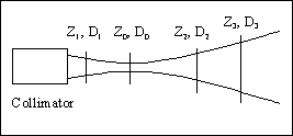
Fig. 3.5: Measurement of beam properties
From optics the actual laser beams satisfy the following equation.
![]() , n=1,2,3.
, n=1,2,3.
Where Dn is the beam size at location Zn, D0 is the beam waist, Z0 is the beam waist location, l is the wavelength, M2 is the beam quality parameter we are looking for. In this relation, l is known, Dn and Zn can be measured, M2, D0 and Z0 are unknowns. Taking the measured data into equation 3.4, we get three highly nonlinear equations for three unknowns. One can solve these equations using Mathematica 4.0. Using the above equation, konwing M, beam diameter at any location on the optical axis can be calculated. This is useful for real time focus control.
Knowing M2, one can quickly calculate the beam divergence, focused spot size and depth of focus (DOF).
![]()
![]()
![]()
![]()
![]()
Where DL is the laser beam size when it propagates to the front side of the focus objective lens, f is the focus length, Dmin is the minimum beam diameter that can be achieved. q act is the real beam divergence.
 Example:
Measured data Z1 = (2 + 5/32)*25.4mm, D1 = 0.1165*25.4
mm, Z2 = 39.0*25.4mm, D2 = 0.1195*25.4 mm, Z3
= 80.0*25.4mm, D3 = 0.1235*25.4 mm, with l =355nm, f=20mm, we
got the following results:
Example:
Measured data Z1 = (2 + 5/32)*25.4mm, D1 = 0.1165*25.4
mm, Z2 = 39.0*25.4mm, D2 = 0.1195*25.4 mm, Z3
= 80.0*25.4mm, D3 = 0.1235*25.4 mm, with l =355nm, f=20mm, we
got the following results:
Beam waist and location from chosen point: D0 = 2.81774 mm; z0 = -3.70742m;
Beam quality: M = 1.22366; M2=1.49735;
Beam size and divergence: DL=2.96933mm; Dmin=4.55768*10-6m;
q act=60.05*10-6rad, q Gaussian=40.10*10-6rad, q infinity=44.96*10-6rad;
DOF=± 9.8215*10-6m.
It can be verified that the equations are solved with an error less than 10-10.
In summary, we first measure the pulse energy or average power of the laser beam, then measure the beam spot size along the optical axis. Using equation (3.4) we can calculate the beam waist and beam waist location, and we can find M2 of the beam, then we can calculate the other indexes in equation (3.5). Knowing diameter at any location, we can find out the intensity. Finally we combine the spatial and temporal distribution of the laser energy, we get the most general form of laser energy model:
![]()
Where I0(t, z) is function of time and distance from beam waist z, SP(x,y) is the spatial distribution of laser energy and it is a function of x and y. SP may take forms other than Gaussian distribution, we can even integrate complex spatial modulation into this function, for example, pattern information in texturing can be embed in this function.
Next we will discuss laser energy absorption by the target material.
![]()
![]()